Description of the AA-Methods
First I am going to shortly characterize the "old" antialiasing methods
currently used with POV-Ray. For a more detailed description see the
manual or the source code (render.c).
Method 1
Method one takes for each pixel a sample in the middle of the pixel. Then
if the resulting colour differs more than threshold from the (previously
calculated) colour of the left or of the upper neighbour pixel supersampling
is done. Not only the current pixel is supersampled but also the neighbour
to which the colour difference has been (if this had not already been done
perviously).
For supersampling samples are taken in a fixed nxn grid where
n=AntialiasDepth. The average of all samples becomes the pixel's new
colour.
Advantages: - The method affects very directly the visibility as supersampling
is only done if there were a visible colour change in the picture. - The numbers
of samples per pixels is usually kept at a moderate rate. - Supersampling of one
pixel can also affect its (already traced) neighbours. Therefore a aliasing
effect discovered only in the next line will correct the upper line.
Disadvantages: - The last point mentioned as advantage is limited. Only the
line just above and the pixel left to the current can be changed. This leads
to the effect that thin lines going from upper-left to lower-right come out
better than other. You clearly see this assymetrie in
test scene 2. - Objects smaller than a pixel are only caught randomly.
- The number of samples does not scale with the difficulty
of the aliasing effect. If supersampling is done there are always n^2 samples
taken -- no matter of how big the colour difference were or how the supersamples
are
Method 2
Method two takes samples at the four corners of each pixel (as all corners of
non-border pixels are shared by four pixels there is still only one sample per pixel
for not too tiny pictures). Then there is checked if the corners' colours differ
more than threshold from each other. If so supersampling is done by
dividing the pixel in four subpixels and for each subpixel a call to the
trace_sub_pixel function is made. This function samples all the corners
of the subpixel and then -- as with the pixel itself -- checks if there
is a colour difference and calls itself recursively if so (and the maximum
depth has not already been reached).
Advantages: - Scales with the complexity of the alias effect.
Disadvantages: - Quickly leads to a high number of samples taken. - Does
extreamly bad with thin lines. - Objects smaller than a pixel are only caught randomly.
- See method 3-5 for further improvable things.
All my new methods are based on the second, adaptive method. That means they
all go for the samples at the pixels' corners first and decide then what to do.
These methods therefore are in first line thought as replacement/improvement to
method 2. In the used test scenes method 3/4 have shown to always perform
equally or better than method 2. Of course there could be a scene constructed
which showed the opposite.
Method 3
Method 2 does not consider if big parts of the pixel are supersampled or
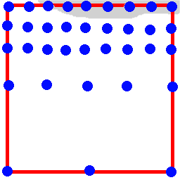
only a small part. Have a look at this example:

The red box marks a pixel. Blue points mark sample taken with method 2, depth 3
if the difference of the grey to the white is more than the threshold. However
it does not matter if the threshold is much below that or just a bit.
Always 35 samples are taken for supersampling this pixel. Why taking so much samples
when there is quickly clear that the lower part is white anyways and the
upperpart cannot significantly contribute to the colour? However method 2
does not know about the lower part when it starts supersampling in the upper left.
Method 3 does differently. It does not go depth-first but one depth after the
other. So in this example it will trace the 9 points for depth 1. Then it sees
that the lower part will not change any more. Because of this it multiplies
the threshold value by a factor 2! Now it checks again if the colour
difference in the upper part is more than threshold. If not it stops. The idea
behind this is: only continue taking additional samples if the still-changing-area
can change the pixels colour more than (the orginial) threshold. Like this,
method 3 is sensitive to how much above the threshold the colour difference is.
Generally it always multiplies the original threshold by the factor
(pixels area)/(area that will not change any more) before proceeding to the next
depth.
This is the only difference between method 3 and 2. The same strategy
of increasing the threshold while going deeper into recursion is also
used for method 4 and 5.
Method 4
Method 4 is more conservative in taking additional samples. If the corners'
colour differ it does not - like method 2&3 - take 5 additional samples but
only one in the middle of the picture. Then it checks again if the corner
pixels differ from the middle pixel and takes samples on the border line
if they do. This can save us from taken some unneccessary samples.
considering thin lines
If you have looked at the sample scenes you will have seen that
method 4 does considerable better than method 2/3 what conserns the
sampling of thin lines. One could expect that I have combined method 1 and 3
to get this result. This would be possible but is not the case.
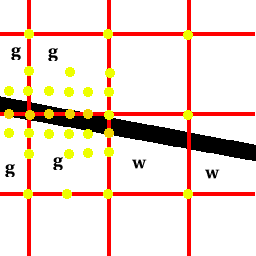
Let's have a look at how a thin line crosses the pixels:

The red grid marks pixel boundaries. The yellow points mark samples that
are taken by the method 4 as described above. The pixels marked with 'g' get
correctly supersampled but the ones with 'w' turn out compleatly white. Method 2
would fail in the same way - even though it takes more samples. How does this
happen? The 'w'-pixels come out compleatly white because the samples at the
corners all miss the line. But from the previous pixel we already know that
a black area is crossing the pixel border as we have supersampled that pixel.
We can use this information! That is what method 4 does. If it has to
check if the colour difference between two points is greater than the
treshold it does not only consider the samples at the two points but
also all the samples which have already been previously taken on the
line between the two points.
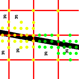
Like that it catchs thin lines similarly to method 1:

And like method 1 it does better with lines going from upper left to lower right.
Method 5
Method 5 is the same as method 4 but it always takes not only samples at the
corner but also the one in the middle of the pixel. This leads to a
samples per pixel ratio of >2 even when the picture is totally black. Why
not have other methods which always take 4,8,.. or more samples with each pixel?
This is not really neccessary because you can always render the picture
n times bigger and scaling it down afterwars hence forcing a minimum of
n^2 pixels per sample. But taking the samples at the corner and the midpoint
has the advantage that the thinnest non-caught line is halfed where the
pps ratio is only doubled. (To archive the same thing with method 4 you have
to render it at double size which results at a minimum of 4pps.)
